Playing with fitness data using Pandas

Published on 05-08-2020 | By Jasdeep Garcha

Running has never been enjoyable. As someone that excelled at team sports, running was always a punishment. As I got older, it has become one of the only outlets I’ve consistently come back to in order to stay fit.

Recently I purchased a GPS watch, primarily in anticipation for this summer because I’d like to see my exertion while hiking. In the meantime, I’ve used it a good bit for running. I’ve never really had this type of insight into my heart rate, cadence, and general fitness, so after logging a dozen or so runs, it seemed like a fun data set to practice using Pandas with.

I’ve observed over the last month a couple of things: 1) I’ve started to enjoy running a bit more, and 2) I’ve been able to run slightly longer distances than I’d ever consider doing in the past (e.g. 4.5+ miles).

What I wanted to do was to see if there were any differences in my longer tracked runs vs. my shorter tracked runs. In other words, are there any differences in my heart rate and/or cadence (two major metrics the watch reports on) between my short runs and my long runs?

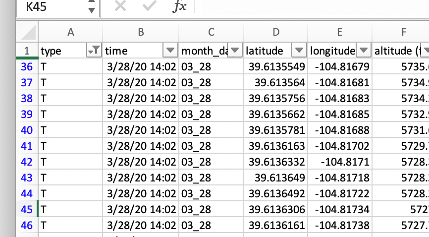
The first challenge was downloading the data. Unfortunately Garmin doesn’t let consumers use their API (huge product gap). Services that are allowed to use their API are a bit more friendly. I used SmashRun to sync my runs from my watch and they generated a .tcx of my run data for me. TCX files are not that useful for data analysis (it seems to be a format meant for mapping software like Google Earth and Strava), so I converted that file into a CSV using GPSVisualizer (surprisingly easy to use).

Once I had the CSV I was ready to start digging into the data a bit more. I fired up a Jupyter notebook to import the data and started to manipulate it there.

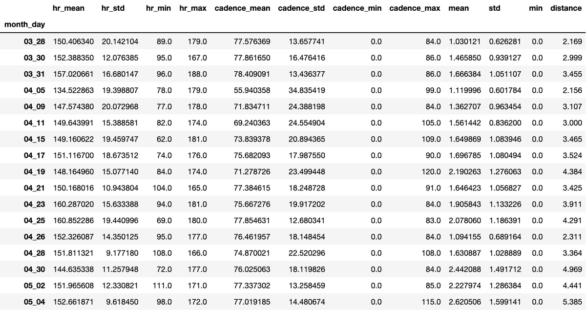
To start, I grouped by run to summarize heart rate and cadence by a few aggregations.

summary_stats = running_data.groupby(['month_day']).agg(["mean","std","min","max"])

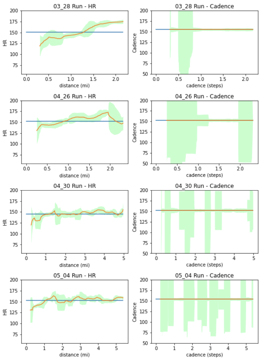
Historically, I’ve only run shorter distances, so I filtered the data down to my two shortest runs to try to isolate a base state (what I had been doing before) and I picked my two longest runs to see what I’m doing now. I then smoothed out the data over rolling 0.25 mile windows, and plotted that over the distance of the run.

run_days = ['03_28','04_26','04_30','05_04']
i=1
fig = plt.figure(figsize=(8,16))
for num, name in enumerate(run_days, start=1):
    ax1 = fig.add_subplot(6,2,i)
    ax1.set(ylim=(55,200))
    plt.plot(result[result.month_day==name]['distance (mi)'],result[result.month_day==name]['hr_mean'])
    hr_mean = result[result.month_day==name]['hr'].rolling(50).mean();
    hr_stdev = result[result.month_day==name]['hr'].rolling(50).std();
    plt.plot(result[result.month_day==name]['distance (mi)'],hr_mean)
    plt.fill_between(result[result.month_day==name]['distance (mi)'],
                     hr_mean-hr_stdev*2,
                     hr_mean+hr_stdev*2,
                     alpha=.5, edgecolor='#3F7F4C', facecolor='#7EFF99',linewidth=0)
    plt.title(name + ' Run - HR')
    plt.xlabel('distance (mi)')
    plt.ylabel('HR')
    ax2 = fig.add_subplot(6,2,i+1)
    ax2.set(ylim=(50,200))
    plt.plot(result[result.month_day==name]['distance (mi)'],result[result.month_day==name]['cadence_mean']*2)
    cadence_mean = result[result.month_day==name]['cadence_mean'].rolling(50).mean()*2;
    cadence_stdev = result[result.month_day==name]['cadence'].rolling(50).std()*2;
    plt.plot(result[result.month_day==name]['distance (mi)'],cadence_mean)
    plt.fill_between(result[result.month_day==name]['distance (mi)'],
                     cadence_mean-cadence_stdev*2,
                     cadence_mean+cadence_stdev*2,
                     alpha=.5, edgecolor='#3F7F4C', facecolor='#7EFF99',linewidth=0)
    plt.plot()
    plt.title(name + ' Run - Cadence')
    plt.xlabel('cadence (steps)')
    plt.ylabel('Cadence')
    i+=2
fig.tight_layout()

The red line is the rolling average, the green area is the standard deviation range, and the blue line is my average heart rate over the entirety of the run.

Cadence is uninteresting, but what’s apparent is my shorter runs have bigger variations in my heart rate, and my longer runs have a much narrower band over the duration of the run.

Looking at that data in tabular form (03_28/04_26 are short runs, 04_30/05_04 are longer runs), you can see the difference clearly in the hr_std column - the standard deviation is tighter on longer runs.

Based on the visualization, the first mile is often an outlier (~150 samples in) as heart rate generally ramps during that period, so I filtered that out for all runs, and you can see the separation between the two sets much more clearly.

run_days = ['03_28','04_26','04_30','05_04']
i=1
after_warmup = pd.DataFrame()
for num, name in enumerate(run_days, start=1):
    after_warmup = after_warmup.append(result[result.month_day==name][150:])

running_data_after_warmup = after_warmup[['type','time','month_day','distance (mi)','speed (mph)','hr','cadence']]
summary_stats_after_warmup = running_data_after_warmup.groupby("month_day").agg(["mean","std","min","max"])
flattened_data_after_warmup = pd.merge(summary_stats_after_warmup['hr'].rename(columns={"mean":"hr_mean","std":"hr_std","min":"hr_min","max":"hr_max"}),
                          summary_stats_after_warmup['cadence'].rename(columns={"mean":"cadence_mean","std":"cadence_std","min":"cadence_min","max":"cadence_max"}),
                          how='left',on='month_day')
flattened_data_after_warmup = pd.merge(flattened_data_after_warmup,
                          summary_stats_after_warmup['distance (mi)'].rename(columns={"max":"distance"}),
                          how='left',on='month_day')
summary_flat_after_warmup = flattened_data_after_warmup[['hr_mean','hr_std','hr_min','hr_max','cadence_mean','cadence_std','cadence_max','distance']]

Of course, this is a somewhat narrow (maybe biased) analysis. In fact, if you look at all runs in the table at the beginning of this post, you may find some longer runs with standard deviations closer to shorter runs. Still, I think there’s some significance in claiming that regulating my heart rate during a run so it stays within a narrower band has some impact on my ability to run longer distances - it sure feels that way!